Convert Structural model to Analysis model

The goal of the Convert Structural model to Analysis model (S2A) workflow is to create an analytical model that can be imported into your analysis software (SCIA Engineer, etc.). The process is divided into 7 steps:

1. Select Model

2. Clean the Model

3. Recognizer Settings

4. Recognizer

5. Alignment Settings

6. Align Elements

7. Saving and Exporting the Model

In every step, the ALLPLAN AutoConverter user can affect the analysis model in various ways. Before starting the S2A workflow you need to have first uploaded the IFC model into ALLPLAN AutoConverter. To begin the workflow, please select Convert Structural model to Analysis model from the Workflow selection bar.

1. Select Model

General objective: Select a model you want to convert to an analysis model.

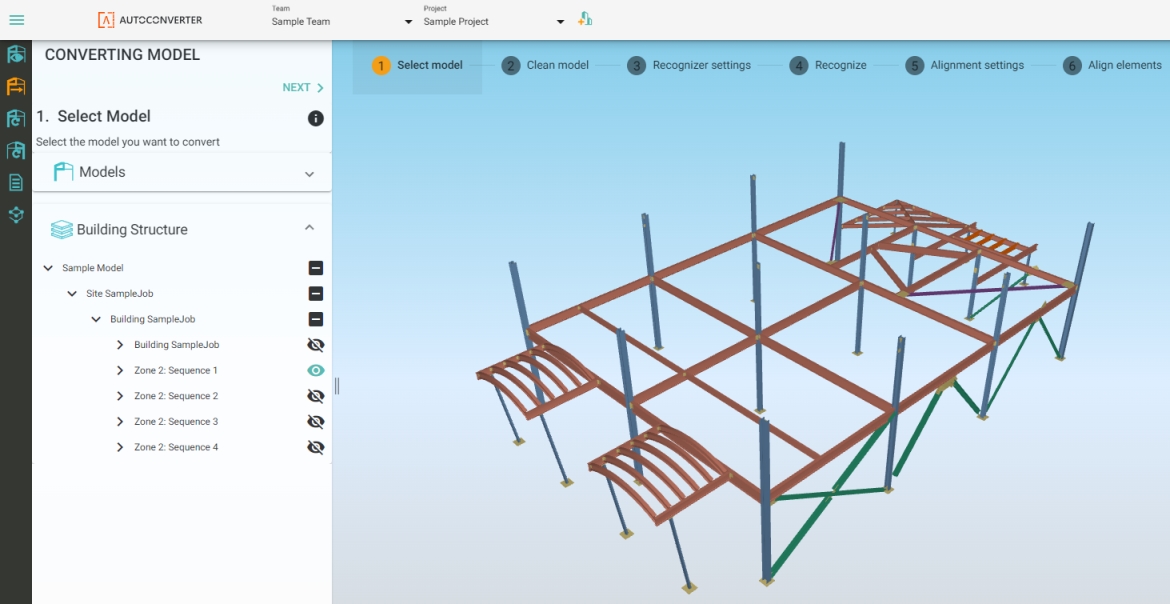
Model selection is done simply by making the model active in the scene. Activate the model by clicking on the eye icon found on the Converting Model workflow tab > Building Structure menu. (Figure 9).

Best practices:

• Activate only one model at a time. Working with multiple structural models at the same time is not currently supported.

• Existing/stored analysis models in AutoConverter can’t be used in this workflow again.

• The model structure often contains multiple disciplines. Activate only the relevant disciplines (building, steel etc.) to streamline the workflow. For one example, filtering to include only the load-bearing structure will make the next step easier.

• IFC models often contain information known as a storey (IfcBuildingStorey). Use the Building Structure menu for fast pre-selection of one or more specific storeys (Figure 9).

2. Clean the Model

General objective: Keep only those objects in the 3D scene that you want to convert to analysis elements.

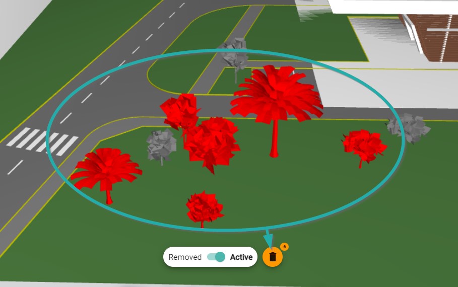
The Clean step is crucial for all further steps. In most cases, we want to convert only the load-bearing structure or part of the load-bearing structure in the 3D scene. To achieve that, you can use the available filtering options. Filtering divides elements into the Active and Removed state. The toggle for switching between Active and Removed is found right above the View settings in the 3D scene (Figure 10).

Filtering in 3D scene:

Filtering in 3D scene (Figure 10) can be easily done by selecting an object. The selected object can be removed by clicking on the trash can icon right above the scene settings component. You can select multiple objects by holding Ctrl + left-click on more objects in 3D scene. Another option for selection is holding Ctrl + left-click + drag to draw a window around objects inside the 3D scene. Every object with a centroid inside the selection window will be selected. The most effective way is to use attribute selection for filtering. Select an object in the 3D scene and take a look at the Properties panel on the right-hand side of the screen. By clicking on the selected property you will achieve a property selection. All objects associated with the selected property and value will be selected in the 3D scene and highlighted.

Active/Removed views:

Everything you remove from the scene with the methods mentioned above can be seen in 3D scene when you switch between an Active and Removed view. The default view is Active. Switch to the Removed view using the toggle above View settings (next to the trash can icon). The Removed view will show all removed elements in the scene. In case you find an element that is considered load-bearing, you can easily move it back to Active using the Keep selected for recognition button (green-colored trashcan icon with an upward-pointing arrow, Figure 11).

IFC Types:

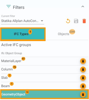
IFC Types offers a raw filtering approach. The IFC Types filter is available on the Workflow specific panel (Figure 12). Click on the trash can icon next to an Object Group to remove it from the scene. Before removing a complete Object Group, you can click on the group to highlight it in the scene. This can help you determine if all of the objects are candidates for removal.

Saving the filter:

The current state of your 3D scene—meaning the state of objects being Active or Removed—can be stored as a saved filter using the save icon as can be seen on Figure 13, left. You will be asked to name the filter, and then the filter is saved. You can load saved filters every time you open the model. One model can have multiple filters stored. Filters can be loaded, updated, and saved again.

Reset filters will activate all removed objects and put the structure in a default state with no active filter.

Delete currently selected filter will permanently delete the active filter. Be careful with deleting filters that might be useful. Filters are also used in other workflows, therefore it is wise to save them.

Best practices:

• Before you start with cleaning, take a look at the available properties in the Properties panel. Look for properties that will help you with the cleaning.

• Examples of useful attributes for filtering:

  LoadBearing = YES or NO. With the LoadBearing attribute correctly set you can easily select all non-loadbearing elements and remove them.

  Material = MineralWool, EPS, etc. With the materials properly defined, you can easily identify non-load bearing elements based on material and remove them.

• You can use inverted selection in case you need to select exactly the opposite objects with the attribute selection.

• Use the Building Structure menu in case it is defined in your IFC file. Going throughout the building storey by storey makes all non-loadbearing elements easy to be removed from the scene.

• During the filtering process, you can also use functions available in the View settings of the 3D scene, especially the Hide and Invert Selection functions.

3. Recognizer Settings

General objective of the step: Define how the active objects in the scene should be handled by the Recognizer.

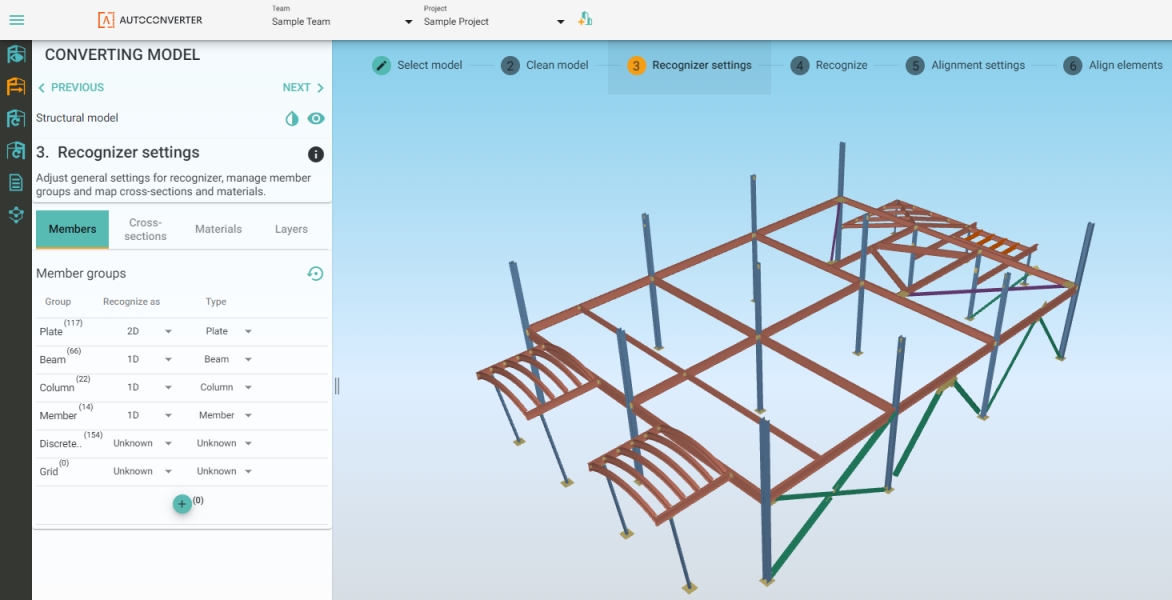
Recognize is a function responsible for converting structural objects into analysis objects. You can set the Recognize as setting for each conversion group to 1D, 2D, or Solid. You can assign crosssections for steel and aluminum profiles. You can assign materials from the material library and define layers where possible. This step is also very important for the final model quality. Correctly set dimensions, material, and profiles will increase model quality and save you a lot of time (Figure 14).

Members:

In the Members settings, you can decide how each object group is recognized and converted to an analysis object. By default, several editable groups are created based on the IFCBuildElement entity (typically Beam, Slab, Column, etc.). Elements can be moved to the newly defined groups and between existing groups. This provides you with flexibility in case the IFC data does not conform to structural reality. The group component is divided into 3 columns: Group, Recognize as, and Type. Each row represents a separate group. Every object in the 3D scene can be assigned to only one group.

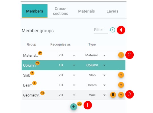
Member groups component buttons (Figure 15):

(1) Create new group: New groups can be created as empty or with a selection of elements.

(2) Add elements to an existing group: When you have a selection of elements you can reassign them to another existing group.

(3) Delete group: Existing group will be deleted and a new Not assigned group will be created. All elements have to be in the recognition group.

(4) Restore defaults: The groups will be reset to a default IFC structure-based state.

Member groups component columns (Figure 15):

• Group contains the name of each group along with the number of entities assigned to the specific group. Groups can easily be renamed by double left-clicking on the name. After renaming, confirm the action by pressing Enter .

• Recognized as determines how the structural element will be displayed in the converted group. There are four display options:

  1. Unknown: The algorithm will determine whether an object is 1D, 2D, or solid.

  2. 1D: Elements are displayed as center-lines (typically columns, beams, girders, purlins, rafters, etc.).

  3. 2D: Elements are displayed as center-planes (typically walls, slab, shear walls etc.).

  4. Solids: The Recognizer will not convert elements assigned to this group. The original structural object will be kept and passed to the analysis software as a 3D solid. This can be useful for objects that are not load-bearing but could be of interest (e.g., for defining loads). If you have complex objects like double-curved elements that can’t be recognized, they can be passed to your analysis software and used as a reference.

• Type offers various options for further specification of elements. The selected type is stored and will be transferred to your structural analysis application. Types can also affect the direction of recognition in cases where it is not clear which direction is dominant. This is useful when you have an element you would like to be recognized as 1D, but it has no dominant dimension (meaning, l»a>b). Type then can be decisive in center-line placement.

  • Column: the center-line is primarily vertical.

  • Beam: the center-line is primarily horizontal (in case dimensions are not geometrically clear).

Cross-sections:

Cross-sections settings are dedicated to 1D elements and their profiles (cross-sections). ALLPLAN AutoConverter is capable of recognizing general cross-sections described by polygons, parametric cross-sections (rectangle and circle), and also provides the option for mapping structural profiles to the analysis profile library (HEA, HEM, HEB, IPE, UPE etc.). ALLPLAN AutoConverter can also recognize several compound cross-sections (double-I, double-channel, double-angle, etc.) and compound general cross-sections (see Recognizer).

For setting cross-sections properly before the recognition (the conversion elements from structural to analysis), follow the steps described below. Before you begin, determine if this setting is relevant to your current project. In case you do not have manufactured profiles in your project (e.g., your project is purely concrete elements or timber), you can skip this step and go directly to Materials. All elements are recognized by default as Parametric where possible and as General in all other cases.

In case you have manufactured profiles:

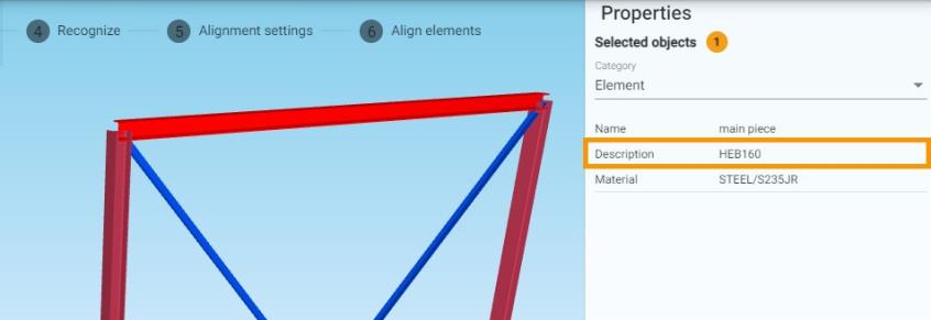
(1) Find the attribute that is containing the cross-section name like HEB160. Inspect elements in your structural model to a find a property that contains data about cross-sections (Figure 16).

(2) Open a property dialogue and select the property that you have identified as the right one for cross-section mapping (Figure 17).

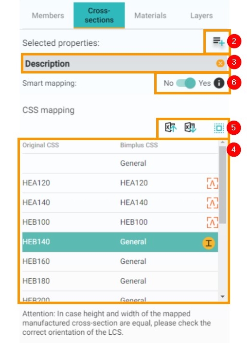
(3) A property will appear in the property list. One or more properties can be selected. In some cases, there might be more suitable attributes for mapping. In case more attributes are selected, the order is important. The second attribute and each subsequent attribute are displayed in the mapping table as rows for elements that have no value for the hierarchically superior attributes. This eliminates the issue with "double" mapping, but still provides you flexibility in profile mapping.

(4) The mapping table is shown when the attribute is selected. The table has two columns and one action. The Original CSS column represents the value from the structural model. The Bimplus CSS column represents the value from the steel profile library (default value is General). The action button is shown when the row is selected, and is used for the mapping to the steel profile library available in ALLPLAN AutoConverter.

(5) Other action buttons: There is an option for Microsoft Excel mapping. Import is for loading the mapping table inside ALLPLAN AutoConverter. Export is for exporting a mapping table from ALLPLAN AutoConverter to an Excel sheet. Excel mapping can save you time during the mapping. You can export to Excel, do the mapping manually in Excel, save it, and import the Excel file back into the ALLPLAN AutoConverter. You can also reuse your mapping table across multiple projects in ALLPLAN AutoConverter by exporting it from one project and importing it into a different project.

(6) Smart mapping toggle: Smart mapping toggle helps you make the mapping process faster. When toggled ON, it tries to find a logic in the mapping you provided. In case you map IPE_200 to IPE200 profile from the library, Smart mapping will automatically map all others IPE_*** to IPE***.

Mapping dialogue:

The Mapping dialogue can be opened by clicking on the action icon in the selected row in the mapping table (Figure 16). In the dialogue, first select a type. When the type is set to General, the algorithm will recognize a shape and will create either a general or a parametric cross-section where possible. When the type is set to Manufactured - rolled, Manufactured - welded, or Manufactured - cold formed, the dialog will guide you through the library tree to the final cross-section that is defined in the AutoConverter steel profile library. For example: When Manufactured - rolled is the type, I-section is the category, and HEB is the cross-section group, HEB140 will be the final library profile.

The special Type in the mapping dialogue is Manufactured - user defined. With this type of CSS, you are not limited to the library available in the ALLPLAN AutoConverter. By using the Manufactured - user defined type, you can define your own manufactured type of cross-section that is familiar to your analysis software.

How to define a User defined manufactured cross-section (Figure 18):

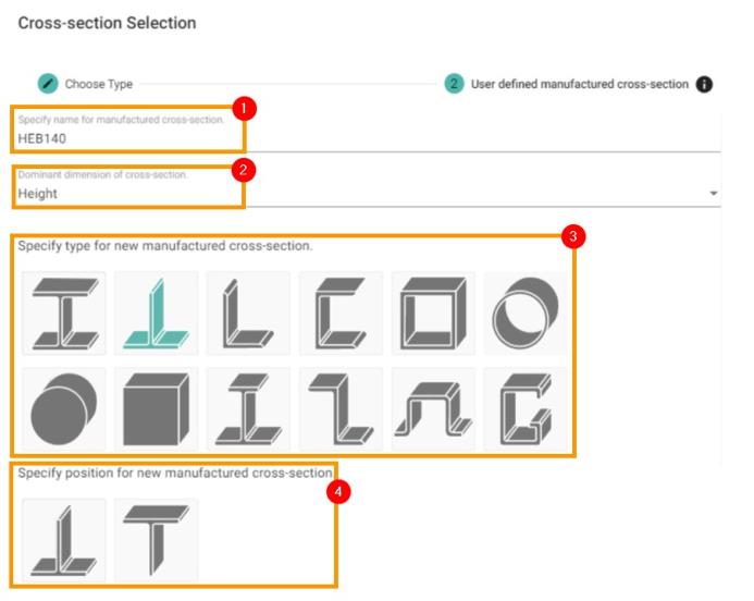
(1) Specify a name. This should be a name known in your analysis software cross-section library.

(2) Set the dominant dimension. Usually, it is a height. This is necessary for the correct positioning of the profile and local coordinate system in relation with the bounding box of the cross-section.

(3) Set the type of profile you are now defining.

(4) Select formcode when necessary. More about formcode can be found in the saf.guide - formcodes. Formcodes are important in defining certain profiles the cross-section library in relation to the member’s local coordinate system. For profiles with two axes of symmetry, formcodes are irrelevant. For profiles with one axis of symmetry there are two formcode options (typically asymmetric I sections they can be placed with wider flange in local Z positive or local Z negative). Profiles with no axis of symmetry typically have four formcodes (L-sections for example).

Materials:

Mapping of the materials is, in principle, the same as the mapping of the cross-section. The goal is to assign correct materials to members based on attribute mapping. When no action is taken in this step, all members are assigned with default material MAT1. This material is not suitable for analysis and manual change is necessary in your analysis software. It is recommended to map material where possible and thus save yourself time spend with manual reassignment.

How to map materials?

1. Select a property useful for mapping.

2. The property is shown in the Selected properties list. Similar to cross-sections, there might be more properties selected with the same rules.

3. Map the structural attribute to the material library using the action button that shows up after the selection.

For a more detailed description of action buttons please refer to cross-sections, where the functionality is the same.

Layers:

Mapping of layers is, in principle, the same as material mapping and cross-section mapping. The key is to select a useful property and map it to the desired value. The only difference is that there is no library and you can set the value as you wish. In case layers are not defined, a basic layer set is created based on the type of object available in SAF (saf.guide). For example, the StructuralCurveMember layer for all 1D elements, StructuralSuraceMember for all 2D elements etc.

How to define layers (Figure 19): 

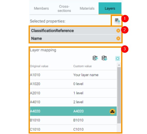
Figure 19: Layers definition

(1) Select a property that is useful for mapping.

(2) Property is shown on the Selected properties list. Similar to cross-section and materials, there might be more properties selected with same rules.

(3) Layer names default to the same value as the selected property. You can change it to your own specified name by clicking on the action button a typing the new name in.

When you are satisfied with the Recognizer settings, you can proceed to the next step: Recognizer.

4. Recognizer

The Recognizer is the step where the conversion takes place from structural objects to analysis objects. Tasks related to object grouping and mapping are done thanks to the previous step, and the last thing we need to do is define the general recognition settings (conversion to analysis objects) and steer the algorithm settings. General settings for Recognizer are found under the gear wheel icon, which consist of:

• Recognition of 1D members: algorithmic rules for 1D conversion.

• Recognition of 2D members: algorithmic rules for 2D conversion.

• Use prefix: rule for the naming of the nodes.

• Support for large models: algorithmic approach towards the recognition process based on model size and complexity

General recognize settings (Figure 20):

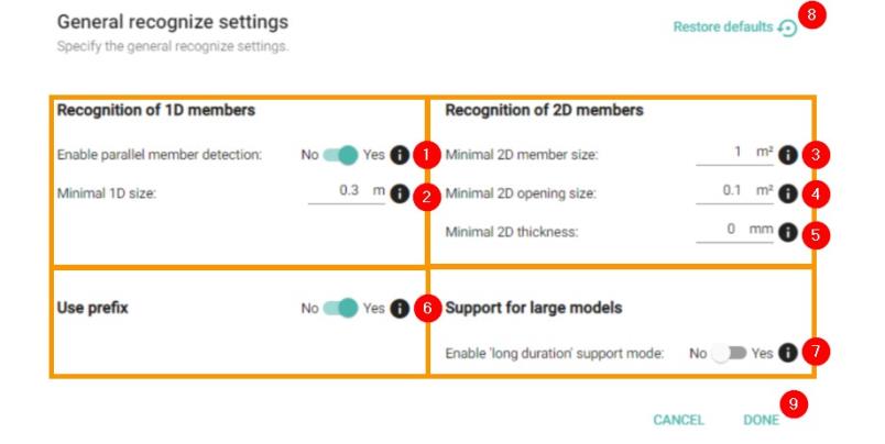
Figure 20: General settings for Recognizer

(1) Enable parallel member detection (toggle): When turned ON, parallel members are detected and the algorithm creates compound cross-sections out of them or general compound cross-sections. Higher priority is placed on the compound cross-section type (for example, double I section, angle back-to-back, etc.) than then general compound cross-section type. See Annexes for the list of supported compound sections, rules, and further information about the general compound type.

(2) Minimal 1D size: Set a rule for minimal 1D length size. All 1D members with lengths smaller than the set value will be placed in a special group after the recognition called Small 1D Members. You can then decide if you want to keep them in your analysis model or remove them. This setting is mainly useful for making sure that the cleaning of the structure was done properly and that there are no forgotten bolts, screws, etc. in your analysis model.

(3) Minimal 2D member size: All 2D elements with smaller area will be placed in a special group called Small 2D Members. After recognition, you can decide which elements you want to keep a which to delete. This might be useful in case you want to be sure all connection plates in steel connections are gone or you have complex 2D element geometry. In some cases where 2D elements have inclined edges, they can have areas with different thicknesses (recesses) or some other complicated geometry, they could be recognized as more than one analysis element. With Minimal 2D member size, you can easily identify them.

(4) Minimal 2D opening size: All openings with an area that is smaller than defined will be placed in the separate group called Small 2D Openings after Recognizer. This allows you to easily get rid of all the small openings in your 2D analysis elements that are irrelevant to the current structural analysis.

(5) Minimal 2D thickness: All 2D elements with a thickness that is smaller than defined will be placed in a separate group called Insufficient thickness. After Recognizer, you can decide which elements to keep in the model and which to remove. This setting might be useful in making sure that all connection plates, plaster boards, etc. are filtered out of the model.

(6) Use prefix (toggle): When set to YES, the naming of the nodes will have a prefix "N" (for example, N101, N102, N103, etc.). When set to NO, nodes will be named only with numbers without the "N" prefix. Verify what the right format for your structural analysis application is. (For SCIA Engineer is recommended to have toggle turned ON.)

(7) Enable long duration support mode (toggle): This applies to a special order of processing structural elements that is effective for huge models only. This processing does not perform well for small or medium size models. In case this needs to be activated, you will be asked for that after the first Recognizer run timeout. The timeout of the regular Recognizer is 2 minutes.

(8) Restore defaults: Recognizer settings are stored in ALLPLAN AutoConverter and are loaded every time you open the model. If you want to restore the default settings, click the Restore defaults button.

(9) Done: All settings are confirmed by clicking on the Done button.

Grouping of elements that do not satisfy conditions set above (Figure 21):

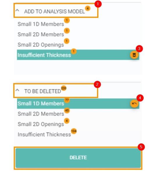
In case some of the recognized objects do not satisfy the Recognizer settings, those objects are placed in separate groups. The above-mentioned groups for specific conditions are (1) Add to analysis model and (2) To be deleted. Below the two main groups, there is one group for each condition in settings Small 1D Members, Small 2D Members, Small 2D Openings, and Insufficient Thickness.

Elements can be moved between the main groups using the action buttons.

Buttons (3) and (4) are available when the whole group is selected or when one or more elements from a specific group are selected. That means you can move all elements at once between groups or you can use selection in the 3D scene for moving only selected objects (openings for Small 2D Openings, 1D members for Small 1D Members, etc.). When you are done with the regrouping between Add to analysis model and To be deleted group press the (5) Delete button. The delete button will remove all elements that are placed under To be deleted and all objects under Add to analysis model will be kept. In normal case, you delete all the To be deleted objects as they have passed your threshold.

Note: Recognizer can also be run with a selection of elements. Selection can be done the usual way: object selection, window selection, and attribute based selection. If you decide to Recognizer this way, keep in mind that you are also defining the selection for the next steps (Alignment setting, Align elements).

5. Alignment Settings

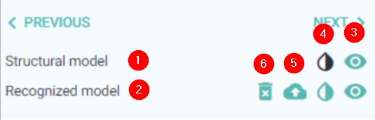
Now you have successfully converted your active objects in the scene. In the model view settings, you can see now two models: The (1) Structural model and the (2) Recognized model. Besides the already known toggle buttons for (3) visibility and (4) transparency, you can see also the new (5) Save recognized model and (6) Delete recognized model on Figure 22.

The general purpose of alignment settings is to prepare everything for the alignment process. The alignment process will connect elements together. Before the alignment takes place, you have the option to adjust the positions of center-lines and center-planes for analytical elements and set which analysis eccentricities you would like to take into account. Also, in the Element behavior tab you can enforce the master planes and prevent elements from movement in the alignment process.

System lines:

The System lines component works similar to Members in the Recognizer setting in terms of creating groups and moving elements between groups. In addition, there are rules that 1D analysis elements can be reassigned to a 1D group, and 2D elements to a 2D group. Solids are excluded from grouping and keep a strictly geometrical representation. Every row in System lines groups represents one group. Groups are based on Recognizer settings groups defined by Recognized as and Type.

System lines component (Figure 23):

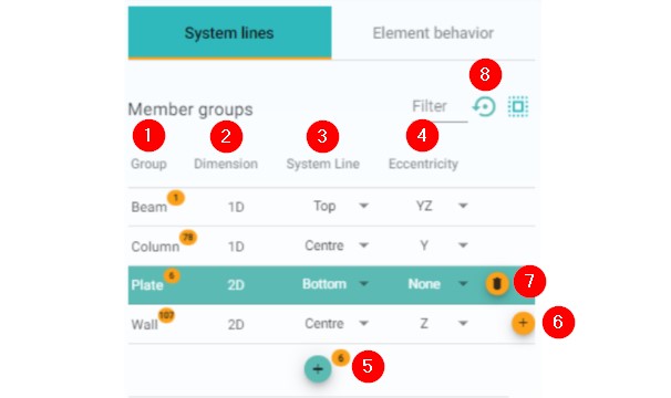
(1) Group: Name of a group. Groups can be renamed the same as a Member group in Recognizer settings.

(2) Dimension: Read-only field that indicates the analysis representation of the group. Typically 1D or 2D.

(3) System line: Drop down selection field that provides you with the option to change the system line position. A list of system line positions is presented in the Annexes.

(4) Eccentricity: Drop down selection field. In case you want to take eccentricities into account in your structural analysis, select the direction from the drop down. Available values are shown in the Annexes.

(5) Create a group: Action button which creates a new group with selected entities. In case, you have both 1D and 2D elements selected, two groups will be created.

(6) Add to group: When selection is done, the object can be reassigned to a group.

(7) Delete group (hover state): On hover, you can delete the group. All objects will be moved to either new or existing group D unassigned.

(8) Restore defaults: Reverts the settings to their original state.

Element behavior:

The Element behavior component is empty by default. The component is used to freeze elements (both 2D and 1D) along the specific axes. 2D elements can be frozen along the local Z axis and 1D elements can be frozen along the Z, Y or both. Freezing the elements will prevent them from moving in the alignment algorithm and all other elements will tend to be connected to them. They will define so-called master planes.

Element behavior component (Figure 24):

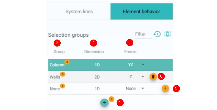
(1) Create a group: Select elements and click on the action button to create a group. Groups will be created based on the type of analysis entity (1D or 2D).

(2) Group column: Name of the group is shown. Groups can have custom names.

(3) Dimension column: Unchangeable value, show the analysis type of entities in the group.

(4) Freeze: A drop-down allows you to choose the direction which an element should be frozen—movement in alignment will be prevented. See the Annexes for available values for Freeze.

(5) Add to another group: By clicking the action button, you can move entities to different groups. Selected objects selected in the scene can also be moved to different groups.

(6) Delete group: The group will be deleted and its entities won’t be frozen anymore.

Best practices:

When you want to change the system line of one beam only, the right approach is to select analysis objects in the 3D scene, create a new group, and set the correct system line position. The same approach is working for eccentricities.

In element behavior, you are usually working with only a few elements that you are choosing for freezing. Freezing means that these elements will not move in the defined direction. It will create a so-called master plane and all elements in relation with this frozen element will move to that master plane. Typical situation for using this freeze option:

• A slab is moved to the plane of a sub-region as this sub-region has a much bigger thickness. Then you freeze that slab and you will see that the sub-regions are moved to the plane of this slab.

• There are different levels for slabs on one floor and you want to keep this difference in height. Then you freeze these slabs.

• There are beams moved to the level of other beams close to them. Then you freeze one member in each plane to keep them both.

You can experience a decrease in the quality of the aligned model when there are too many elements in the freeze state. In that case, it is useful to reset freeze to defaults and start over again and freeze less elements.

6. Align Elements

The main purpose of this step is to connect elements to each other and obtain a valid structural analysis model. Connection is done based on alignment settings and can be done in 3 modes: Align all at once, Partial alignment based on selection, and the more advanced Alignment per groups. General settings (Figure 25 ) steer the algorithm, so understanding the settings is crucial for the alignment result.

General alignment settings:

General alignment settings are a set of values, toggles, and options that will adjust the alignment algorithm rules. These settings have a direct impact on the alignment outcome: which members will be connected, which members won’t be connected, and if the post-processing objects will be created or not (for example intersection objects, subregions, ribs, etc.). You can see the complete alignment settings in Figure 25. Alignments settings consist of several parts, but the two main parts are General alignment settings and Align connection settings.

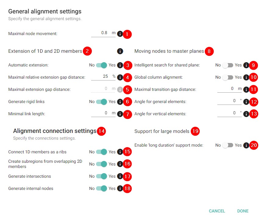
Description of setting values and options (Figure 25):

(1) Maximal node movement: Sets the maximum value for the movement of nodes during the alignment procedure. This value is superior to all other settings and values.

(2) Extension of 1D and 2D elements: These settings determine the behavior of 1D and 2D objects, and their extension during the alignment. Values focus mostly on the structural gap between boundary boxes of 1D elements and faces of 2D elements. Structural objects with overlapping or touching boundary boxes (1D elements) and touching of overlapping masses (2D elements) will be connected automatically to ensure there is no structural gap between them.

(3) Automatic extension (toggle): Defines how the maximal bridged gap should be calculated: either as a relative value to the length of each 1D element and to the thickness of each 2D element (4), or as hard-set values in meters (5).

(4) Maximal relative extension gap distance: Sets the maximum relative gap between recognized member boundary surfaces to be bridged by extension, in relative percentage. This value applies to both ends of the member, and the original length of each member is used as its own reference.

(5) Maximal extension gap distance: Sets the maximum absolute gap between recognized member surfaces to be bridged by extension. This value applies to both ends of the member.

(6) Generate rigid links (toggle): Turn ON or OFF rigid link creation in the alignment process.

(7) Minimal link length: This field is active only when Rigid link creation is toggled ON. When the length of the extension in the alignment of 1D elements is equal or bigger than set value, the rigid link is created instead of the element extension..

(8) Moving nodes to master planes: Settings in this category affect other movements than an extension of the center-line for 1D and edge extension for 2D.

(9) Intelligent search for shared plane (toggle): This toggle defines the position of the plane of analysis elements, typically for rafters and purlins. When toggled ON, master plane is shifted towards the contact plane between rafters and purlins. When turned OFF, master plane is usually defined by rafters (members with the dominant dimension of cross-section boundary box).

(10) Global column alignment (toggle): When turned ON, physically separate structures will share the vertical master planes.

(11) Maximal transition gap distance: Set value that should be bridged during alignment in the movement of 1D elements into common master planes. Value is in meters.

(12) Angle for general elements: Set value in degrees (up to 10°). This value works around small discrepancies in structural models and helps you align elements in straight segments.

(13) Angle for vertical elements: Set value in degrees (up to 10°). This value works around small discrepancies in structural models and helps you align vertical elements in straight segments.

(14) Alignment connection settings: Used for post-processing the aligned model. These settings do not affect the overall model geometry.

(15) Connect 1D members as ribs (toggle): When toggled ON ribs (StructuralCurveMemberRib in SAF) are automatically created. Ribs are separate objects linked to the parent slab. Some structural analysis software allows the creation of ribs afterward when using them, in which case you can keep the toggle turned OFF and create ribs there.

(16) Create sub-regions from overlapping 2D members (toggle): Usually used for mushroom heads above columns or for local stiffening of foundation slabs. When toggled ON, sub-regions (StructuralSurfaceMemberRegion in SAF) are automatically created from overlapping elements. Sub-regions are separate analysis objects linked to the parent slab.

(17) Generate intersections (toggle): When turned ON, internal edges (StructuralCurveEdge in SAF) are created in logical places on 2D analysis elements. Some structural analysis software allows the creation of internal edges afterwards directly when using them, in that case, you can keep the toggle turned OFF.

(18) Generate internal nodes (toggle): When turned ON, nodes logically moved to center-lines and planes of different analysis elements during the alignment process are listed there as internal nodes. This toggle is not related to new object creation, it only stores the reference. Some structural analysis software allows the creation of internal nodes to be referenced afterward, in which case, you can keep the toggle turned OFF.

(19) Support for large models: This setting should be used only in cases when large and geometrically complex models can’t be aligned and the alignment times out.

(20) Enable long duration support model (toggle): Adjusts the alignment data processing. Usually you won’t need to use this toggle. In case you have huge models, you will be asked by ALLPLAN AutoConverter to turn it ON after the timeout of the first alignment attempt (timeout occurs approximately after 2 minutes).

Partial alignment:

Now we have finished the settings we can press the alignment button and the whole model will be aligned. There are situations that you want to align step-by-step. This is possible by selecting recognized objects in the 3D scene. You will see that the Align button is changed to a Partial Alignment button. Once done you can change the settings and select another group of recognized objects. If you make a mistake you have to start all over again. You will also have to start over if you changed the settings in between partial alignments. There is a more advanced way of doing this by using the Alignment per groups which is explained next.

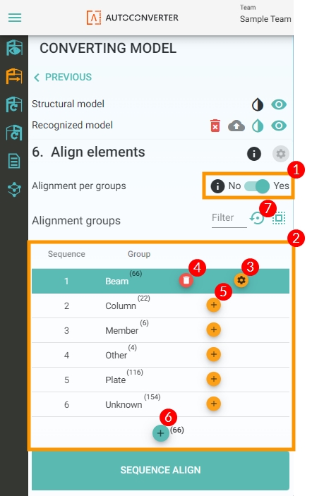
Alignment per groups (Figure 26):

Alignment per groups is an alignment procedure where recognized elements are placed in groups and aligned in sequence, one group after another. You can activate the feature by toggling ON the Alignment per groups (1).

The grouping component (2) is activated. Each group has its own alignment settings (3) which allow you to steer the alignment procedure in a very detailed way; allowing you to take into consideration the specific needs of the individual parts of your structure. Working with the groups is consistent with other components as well: you can create and delete groups (4), move elements between groups (5), create new groups (6), and reset all to default with the reset button (7). The order of the groups plays a significant role in this step, and can be changed simply by dragging and dropping the group to the desired position. When you are satisfied with the distribution of recognized analysis elements in the groups, the order of groups, and the Alignment settings for every group, you can hit the alignment button.

Alignment is done in the hierarchical order of groups, one after another. You can also align only the selected groups. Click on a group to select it (or use "ctrl + left mouse click" to create a multiple group selection). For the best result, order groups in a way that the 1st group has the highest maximal node movement so this setting is descending group by group. Alignment per groups can significantly improve the quality of the analysis model. Typical examples are: Aligning Beams and Columns in one group, and Braces in the next group, Aligning the subsection of the model based on needs for different settings for maximal node movement (case shown on Figure 26), or Aligning fist walls + slabs and 1D elements in one or more separate groups.

Best practices:

• Always pay attention to the maximal node movement value. A correctly set value significantly reduces the number of unwanted connections.

• Check the tool-tips in the alignment settings, with visual examples in there you will be able to understand each value properly. (Check the tool-tips also in other parts of ALLPLAN AutoConverter).

• When dealing with precast structures, focus on the Extension of 1D (and 2D members) and on Generate rigid link settings.

• When dealing with steel structures, focus on the Extension of 1D (and 2D members) and add on the Maximal transition gap distance.

• If you are not satisfied with the outcome of alignment, try to set Angle for general elements to approximately 3° and check the result again.

• When you have a model with sub-regions, you might need to freeze the main slab in cases when slab aligned as sub-regions has a bigger thickness. When you have an unwanted overlap of objects in the structural model and sub-regions are turned ON in settings, you can use them for the detection of such places and delete them in your structural analysis software in case the overlap is unwanted.

• When you want to create sub-regions in Alignment per groups, please put elements meant for sub-regions to the last group of alignment, otherwise, they won’t proceed to the final aligned model.

Notes:

In case you have beams with width as the dominant dimension of cross-section, and you intend to connect them as ribs, check the position of ribs in your analysis software. Ribs do not have their own local coordinate systems; they are inheriting LCS from the slabs to which they belong and therefore they might be rotated!

7. Saving and Exporting the Model

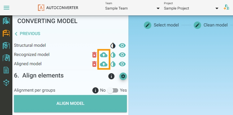
When the model is successfully aligned, it is time to save the model and import it into your analysis software. For saving the model click on the cloud (Figure 27) icon in the model section on the left. After clicking on the cloud icon, the saving dialogue will appear. In saving dialogue you can choose between two options for how to save the model, use either save to Bimplus option or save to .xlsx file in SAF format.

Saving to Bimplus:

The Saving to Bimplus option will save the analysis model on Bimplus servers. After saving, the model will instantly be accessible in the ALLPLAN AutoConverter and in Bimplus. The model can be downloaded to your analysis software via import dialogue dedicated to Bimplus. This approach is recommended to SCIA Engineer users and it brings benefits related to revision handling and the update workflows.

How to save the model to Bimplus (Figure 28):

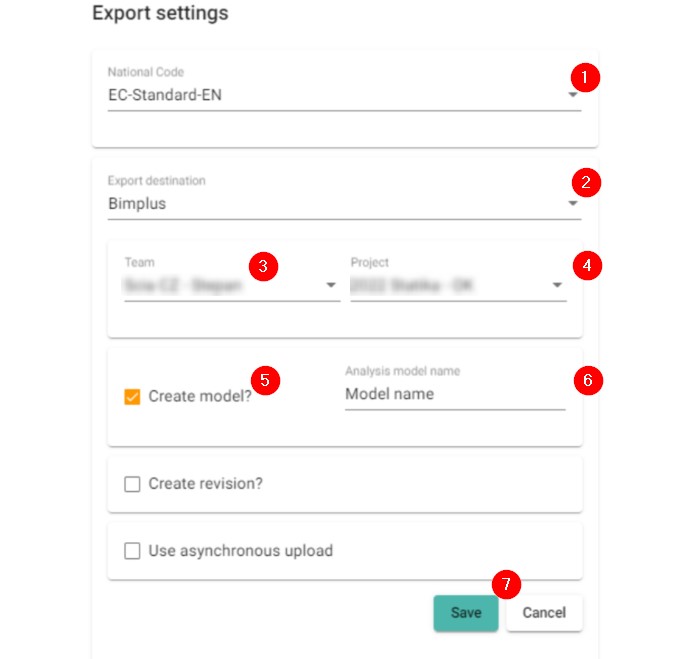
(1) National code: Select the national code you intend to use in your analysis software. The national code can usually be changed in your analysis software afterward (SCIA Engineer).

(2) Export destination: In the drop down select Bimplus.

(3) Team: Select the team in which you want to save the model. Usually, the same team where you have the structural model you have just converted into the analysis model.

(4) Project: Select the project in which you want to save the model. Usually, the same project where you have the structural model you have just converted into the analysis model.

(5) Create model: Check the box if you want to save the model as a new one. Usually used after the first conversion from structural to analysis.

(6) Analysis model name: Give the analysis model a name, which can also be changed on Bimplus at a later time.

(7) Click on the Save button.

How to save a revision on Bimplus (Figure 29):

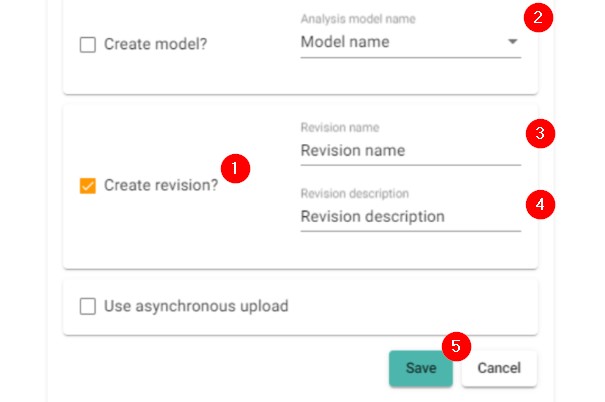
(1) Create a revision: Check the box for saving a model as a revision of an already existing analysis model. Usually used in workflow in Update of an analysis model.

(2) Analysis model name: Select the right analysis model from the drop down.

(3) Revision name: Give a name to a revision you are about to create. The revision name does not need to include the revision number. Revisions are numbered automatically in the ALLPLAN AutoConverter.

(4) Revision description: You can list known changes or any other general text in this field.

(5) Click on the Save button.

Saving to the SAF (.xlsx) file (Figure 30):

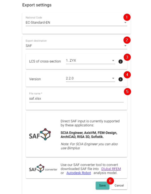
Saving to the SAF file provides you with the option of saving to your local drive. SAF is an open format dedicated to the transfer of structural analysis models. SAF can be imported into your analysis software. SAF files can be viewed and edited by Microsoft Excel or any other software capable of opening the .xlsx files.

How to save a model as an SAF file (Figure 30):

(1) National code: Select the national code you intend to use in your analysis software. National code can usually be changed in your analysis software afterward.

(2) Export destination: Select SAF in the drop-down.

(3) LCS of cross-section: In drop-down, select the LCS of cross-section used in your analysis software. The LCS of cross-section is related to the way cross-sections are stored in local libraries of analysis software. For more info open the tool-tip in ALLPLAN AutoConverter (SCIA Engineer uses "1.ZYX").

(4) Version: Select the SAF version you want to export to. Check first which SAF version is supported in your analysis software.

(5) File name: Give the file the name.

(6) Click on the Save button.